You can run this notebook in a live session or view it on Github.

Parallel and Distributed Machine Learning

Dask-ML has resources for parallel and distributed machine learning.

Types of Scaling

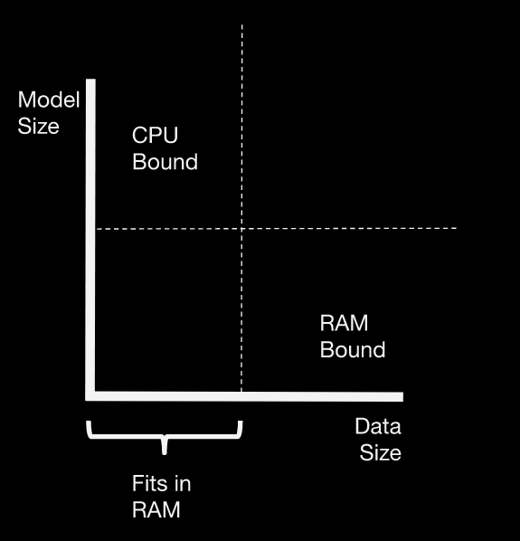
There are a couple of distinct scaling problems you might face. The scaling strategy depends on which problem you’re facing.

1. CPU-Bound: Data fits in RAM, but training takes too long. Many hyperparameter combinations, a large ensemble of many models, etc.

2. Memory-bound: Data is larger than RAM, and sampling isn’t an option.

• For in-memory problems, just use scikit-learn (or your favorite ML library).

• For large models, use dask_ml.joblib and your favorite scikit-learn estimator

• For large datasets, use dask_ml estimators

Scikit-Learn in 5 Minutes

Scikit-Learn has a nice, consistent API.

1. You instantiate an Estimator (e.g. LinearRegression, RandomForestClassifier, etc.). All of the models hyperparameters (user-specified parameters, not the ones learned by the estimator) are passed to the estimator when it’s created.

2. You call estimator.fit(X, y) to train the estimator.

3. Use estimator to inspect attributes, make predictions, etc.

Let’s generate some random data.

from sklearn.datasets import make_classification

X, y = make_classification(n_samples=10000, n_features=4, random_state=0)
X[:8]

y[:8]

We’ll fit a Support Vector Classifier.

from sklearn.svm import SVC

Create the estimator and fit it.

estimator = SVC(random_state=0)
estimator.fit(X, y)

Inspect the learned attributes.

estimator.support_vectors_[:4]

Check the accuracy.

estimator.score(X, y)

Hyperparameters

Most models have hyperparameters. They affect the fit, but are specified up front instead of learned during training.

estimator = SVC(C=0.00001, shrinking=False, random_state=0)
estimator.fit(X, y)
estimator.support_vectors_[:4]

estimator.score(X, y)

Hyperparameter Optimization

There are a few ways to learn the best hyperparameters while training. One is GridSearchCV. As the name implies, this does a brute-force search over a grid of hyperparameter combinations.

from sklearn.model_selection import GridSearchCV

%%time
estimator = SVC(gamma='auto', random_state=0, probability=True)
param_grid = {
    'C': [0.001, 10.0],
    'kernel': ['rbf', 'poly'],
}

grid_search = GridSearchCV(estimator, param_grid, verbose=2, cv=2)
grid_search.fit(X, y)

Single-machine parallelism with scikit-learn

Scikit-Learn has nice single-machine parallelism, via Joblib. Any scikit-learn estimator that can operate in parallel exposes an n_jobs keyword. This controls the number of CPU cores that will be used.

%%time
grid_search = GridSearchCV(estimator, param_grid, verbose=2, cv=2, n_jobs=-1)
grid_search.fit(X, y)

Multi-machine parallelism with Dask

Dask can talk to scikit-learn (via joblib) so that your cluster is used to train a model.

If you run this on a laptop, it will take quite some time, but the CPU usage will be satisfyingly near 100% for the duration. To run faster, you would need a disrtibuted cluster. That would mean putting something in the call to Client something like

c = Client('tcp://my.scheduler.address:8786')

Details on the many ways to create a cluster can be found here.

Let’s try it on a larger problem (more hyperparameters).

import joblib
import dask.distributed

c = dask.distributed.Client()

param_grid = {
    'C': [0.001, 0.1, 1.0, 2.5, 5, 10.0],
    # Uncomment this for larger Grid searches on a cluster
    # 'kernel': ['rbf', 'poly', 'linear'],
    # 'shrinking': [True, False],
}

grid_search = GridSearchCV(estimator, param_grid, verbose=2, cv=5, n_jobs=-1)

%%time
with joblib.parallel_backend("dask", scatter=[X, y]):
    grid_search.fit(X, y)

grid_search.best_params_, grid_search.best_score_

Training on Large Datasets

Sometimes you’ll want to train on a larger than memory dataset. dask-ml has implemented estimators that work well on dask arrays and dataframes that may be larger than your machine’s RAM.

import dask.array as da
import dask.delayed
from sklearn.datasets import make_blobs
import numpy as np

We’ll make a small (random) dataset locally using scikit-learn.

n_centers = 12
n_features = 20

X_small, y_small = make_blobs(n_samples=1000, centers=n_centers, n_features=n_features, random_state=0)

centers = np.zeros((n_centers, n_features))

for i in range(n_centers):
    centers[i] = X_small[y_small == i].mean(0)

centers[:4]

The small dataset will be the template for our large random dataset. We’ll use dask.delayed to adapt sklearn.datasets.make_blobs, so that the actual dataset is being generated on our workers.

n_samples_per_block = 200000
n_blocks = 500

delayeds = [dask.delayed(make_blobs)(n_samples=n_samples_per_block,
                                     centers=centers,
                                     n_features=n_features,
                                     random_state=i)[0]
            for i in range(n_blocks)]
arrays = [da.from_delayed(obj, shape=(n_samples_per_block, n_features), dtype=X.dtype)
          for obj in delayeds]
X = da.concatenate(arrays)
X

X = X.persist()  # Only run this on the cluster.

The algorithms implemented in Dask-ML are scalable. They handle larger-than-memory datasets just fine.

They follow the scikit-learn API, so if you’re familiar with scikit-learn, you’ll feel at home with Dask-ML.

from dask_ml.cluster import KMeans

clf = KMeans(init_max_iter=3, oversampling_factor=10)

%time clf.fit(X)

clf.labels_

clf.labels_[:10].compute()